A 27B-parameter model trained with mixed-precision Adam needs about 16 bytes per parameter: 2 for BF16 weights, 2 for BF16 gradients and 12 for the FP32 master weights and two Adam moments. That is 432 GB before a single activation is stored (activations come later, and they turn out to be just as big). An H200 has 141 GB. So the model has to be split across GPUs, and the question is how.
There are six main ways to split the work, each cutting along a different dimension:
| Method | What it splits | What moves between GPUs |
|---|---|---|
| Data parallelism (DP) and ZeRO | the batch (and, with ZeRO, the optimizer state, gradients and weights) | gradients, sometimes weights |
| Tensor parallelism (TP) | each weight matrix | activations, inside every layer |
| Sequence parallelism (SP) | tokens, between TP’s matrix multiplies | activations, same bytes as TP |
| Context parallelism (CP) | tokens, through the whole layer | keys and values in attention |
| Pipeline parallelism (PP) | layers | activations at stage boundaries |
| Expert parallelism (EP) | the experts of an MoE layer | tokens, all-to-all, in every MoE layer |
This post walks through each one with numbers small enough to check by hand. It follows the papers: Megatron-LM for TP, Korthikanti et al. for SP, Ring Attention for CP, GPipe and its successors for PP, ZeRO, and GShard, Switch Transformer and DeepSeek-V3 for EP.
First: the three collectives
Almost everything below is built from three communication operations. With 2 GPUs and a 4-value vector:
All-reduce: every GPU ends with the full element-wise sum
  GPU 1  [ 1,  2,  3,  4]   ->   [11, 22, 33, 44]
  GPU 2  [10, 20, 30, 40]   ->   [11, 22, 33, 44]

Reduce-scatter: the same sum, but each GPU keeps only its chunk
  GPU 1  [ 1,  2,  3,  4]   ->   [11, 22]
  GPU 2  [10, 20, 30, 40]   ->           [33, 44]

All-gather: each GPU has one chunk; everyone ends with all of them
  GPU 1  [11, 22]           ->   [11, 22, 33, 44]
  GPU 2          [33, 44]   ->   [11, 22, 33, 44]
Two facts to keep in mind:
- All-reduce = reduce-scatter + all-gather. With the ring algorithm on t GPUs and N values, each GPU sends (t − 1)/t · N for a reduce-scatter or an all-gather, and twice that for an all-reduce.
- The backward of a copy is a sum. If a tensor was copied to several GPUs in the forward pass, its gradients must be added in the backward pass. That is why all-gather in forward becomes reduce-scatter in backward, and the other way round.
Data parallelism and ZeRO
Plain data parallelism gives every GPU a full copy of the model and a different slice of the batch. After the backward pass, an all-reduce averages the gradients, and every GPU takes the same optimizer step. It’s simple and scales well, but every GPU still needs all 432 GB.
ZeRO removes that duplication in three stages. Sharding across 8 data-parallel GPUs, for the same 27B model:
| Stage | What is sharded | Bytes per parameter | Per GPU |
|---|---|---|---|
| Plain DP | nothing | 2 + 2 + 12 = 16 | 432 GB |
| ZeRO-1 | optimizer states | 2 + 2 + 12/8 = 5.5 | 148.5 GB |
| ZeRO-2 | + gradients | 2 + 14/8 = 3.75 | 101 GB |
| ZeRO-3 | + weights | 16/8 = 2 | 54 GB |
ZeRO-1 and ZeRO-2 cost no extra traffic: the gradient all-reduce simply becomes a reduce-scatter, followed by an all-gather of the updated weights. ZeRO-3 (the same idea as PyTorch FSDP) also has to all-gather each layer’s weights just before using them, in the forward pass and again in the backward pass, so it moves about 1.5× the bytes of plain DP. Megatron’s --use-distributed-optimizer is roughly ZeRO-1.
ZeRO shards storage. Every GPU still computes every layer on full-size activations. To split the computation itself, you need model parallelism.
What about activations?
The 16 bytes per parameter is only the model state. Activations, the intermediate tensors saved in the forward pass for use in the backward pass, come on top. They scale with tokens, not parameters.
Korthikanti et al. give the activation memory per transformer layer, in bytes, for BF16 with no parallelism and no recomputation:
s·b·h · (34 + 5·a·s/h) s = sequence, b = micro-batch, h = hidden, a = heads
The 34 covers everything linear in sequence length: LayerNorm inputs, Q, K and V, the MLP’s intermediate, dropout masks. The 5·a·s/h term is the attention scores and softmax, which grow with s².
Take a plausible 27B configuration (60 layers, h = 6144, 48 heads; 12·L·h² ≈ 27.2B parameters) and one 4,096-token sequence:
s·b·h = 4096 × 6144 ≈ 25.2M

per layer, linear part:      34 × 25.2M ≈ 0.86 GB
per layer, attention part:  160 × 25.2M ≈ 4.0 GB    (5 × 48 × 4096 / 6144 = 160)

60 layers, naive attention:      ≈ 293 GB per sequence
60 layers, FlashAttention:       ≈ 51 GB per sequence (the s × s scores are never stored)
So a single 4K-token sequence needs activation memory on the same scale as the whole model state, and it grows linearly with the micro-batch size and at least linearly with sequence length. ZeRO doesn’t help here, because every GPU still runs every layer on its full micro-batch. What does help:
- FlashAttention removes the s² term.
- TP with SP, and CP, divide the rest across GPUs (sections below).
- Activation recomputation keeps only each layer’s input (2·sbh) and redoes the forward pass during backward, for about a third more compute.
Tensor parallelism: split every matrix
Megatron-LM (Shoeybi et al., 2019) splits each transformer layer across GPUs with only two all-reduces in the forward pass and two in the backward pass, in plain PyTorch.
The MLP, with real numbers
The MLP computes Z = ReLU(X·A)·B. (Real models use GeLU or SwiGLU; ReLU keeps the arithmetic simple, and any nonlinearity behaves the same way.) Take one token with hidden size 2, MLP width 4, and 2 GPUs:
X = [1, 2]

A = [ 1   0  -1   2 ]        B = [ 1   0 ]
    [ 0   1   1  -1 ]            [ 0   1 ]
                                 [ 1   1 ]
                                 [ 2  -1 ]

One GPU:  X·A = [1, 2, 1, 0]   ReLU -> [1, 2, 1, 0]   ·B -> Z = [2, 3]
Splitting A by rows fails. Give each GPU one row of A and the matching entry of X:
GPU 1:  [1] · [1  0 -1  2]  =  [1, 0, -1,  2]
GPU 2:  [2] · [0  1  1 -1]  =  [0, 2,  2, -2]
                         sum = [1, 2,  1,  0]   correct, but only after adding

ReLU(GPU 1) + ReLU(GPU 2) = [1,0,0,2] + [0,2,2,0] = [1, 2, 2, 2]   wrong
Each GPU holds only a partial sum, and a nonlinearity of partial sums isn’t the nonlinearity of the total. The GPUs would have to all-reduce before every ReLU.
Splitting A by columns works. Both GPUs get all of X, and each computes finished values for its own columns, so ReLU runs locally:
GPU 1:  A1 = [1 0; 0 1]     X·A1 = [1, 2]   ReLU -> Y1 = [1, 2]
GPU 2:  A2 = [-1 2; 1 -1]   X·A2 = [1, 0]   ReLU -> Y2 = [1, 0]
Then split B by rows, so each GPU holds exactly the rows that multiply its half of Y:
GPU 1:  Y1 · B1 = [1, 2] · [1 0; 0 1]    = [1, 2]
GPU 2:  Y2 · B2 = [1, 0] · [1 1; 2 -1]   = [1, 1]
all-reduce:       [1, 2] + [1, 1]        = [2, 3]   = Z on both GPUs
So: column split, then row split, then one all-reduce per MLP block. Each GPU stores half of A and half of B.
The backward pass
Let the loss be L = sum(Z), so ∂L/∂Z = [1, 1]. Each GPU backpropagates through its own half:
through B:     GPU 1: [1,1]·B1ᵀ = [1, 1]      GPU 2: [1,1]·B2ᵀ = [2, 1]
through ReLU:  GPU 1: [1, 1]                  GPU 2: [2, 0]   (input was [1, 0])
through A:     GPU 1: [1,1]·A1ᵀ = [1, 1]      GPU 2: [2,0]·A2ᵀ = [-2, 2]
all-reduce:    [1, 1] + [-2, 2] = [-1, 3]  = ∂L/∂X
X was copied to both GPUs in the forward pass, so its gradient is a sum: the backward-of-a-copy rule again. Megatron calls this the f operator (identity forward, all-reduce backward); the all-reduce after B is the g operator (all-reduce forward, identity backward).
The weight gradients need no tensor-parallel communication at all. ∂L/∂A1 = Xᵀ · ∂L/∂(X·A1), and GPU 1 already has both factors.
Attention
Attention follows the same pattern. W_Q, W_K and W_V are split by columns grouped by head, so each GPU owns whole heads and computes their scores, softmax and weighted sums with no communication. The output projection W_O is split by rows, followed by one all-reduce. Heads must stay whole because a score is a dot product over all of a head’s dimensions; half a head gives half a sum, and softmax can’t be applied to that.
That gives 4 all-reduces per layer: one f and one g for attention, and one of each for the MLP. Because they sit on the critical path of every layer, TP is normally kept inside one node (8 GPUs on NVLink). Two practical limits follow:
- The head count must divide evenly by the TP size.
- With grouped-query attention, 8 KV heads at TP = 16 means each KV head has to be replicated on two GPUs.
Sequence parallelism: the parts TP leaves behind
Megatron-LM duplicates LayerNorm, dropout and the residual add: after g’s all-reduce, every GPU holds the full output and runs these ops on all of it. The compute waste is small, but the activation memory isn’t, because each GPU stores those activations at full size b × s × h.
Sequence parallelism (Korthikanti et al., 2022) splits these ops by tokens. They all treat each token independently, so GPU 1 can take the first half of the sequence and GPU 2 the second, with exact results and no extra communication. (Splitting by the hidden dimension would break LayerNorm, which needs statistics over all h features of each token.)
The trick is that the all-reduce is already a reduce-scatter plus an all-gather, so SP just moves the halves:
X_i (my tokens)          LayerNorm on my tokens         s/2 × h
  | all-gather           (along the sequence)
X (all tokens)           X·A_i -> GeLU -> ·B_i          s × h, partial sums
  | reduce-scatter       (along the sequence)
Z_i (my tokens)          dropout + residual             s/2 × h
Same bytes on the wire as plain TP, and the activations that TP couldn’t split are now divided by t. From the paper’s per-layer formulas (ignoring the attention-score term), TP = 8 alone leaves 10 + 24/8 = 13 · sbh bytes of activations, while TP + SP gives 34/8 ≈ 4.25 · sbh, about 3× less. In Megatron, SP is just --sequence-parallel, and its size always equals the TP size.
Context parallelism: split the sequence through the whole layer
SP splits tokens only between the matrix multiplies, and the weights are still split by TP. Context parallelism splits tokens through the entire layer, and every GPU keeps the full weights. LayerNorm, the projections and the MLP work one token at a time, so they run locally. Attention is the only place where tokens meet.
Take 4 tokens on 2 GPUs: GPU 1 has t1 and t2, GPU 2 has t3 and t4. With a causal mask:
            keys:  t1   t2   t3   t4
query t1  (GPU 1)  x
query t2  (GPU 1)  x    x
query t3  (GPU 2)  x    x    x
query t4  (GPU 2)  x    x    x    x
GPU 2’s queries need keys and values that live on GPU 1. Ring attention passes K/V chunks around a ring of GPUs. At each step, every GPU computes attention for its own queries against the chunk it is holding, while sending that chunk on to the next GPU. With 4 GPUs:
          G1      G2      G3      G4
step 0    K1,V1   K2,V2   K3,V3   K4,V4    <- own chunk
step 1    K4,V4   K1,V1   K2,V2   K3,V3
step 2    K3,V3   K4,V4   K1,V1   K2,V2
step 3    K2,V2   K3,V3   K4,V4   K1,V1
How the softmax stays exact: the online softmax
Each query computes a softmax over keys that arrive in pieces. It keeps three running values: m, the largest score so far; ℓ, the sum of e^(score − m); and o, the sum of e^(score − m) · v. When the max rises, rescale the old ℓ and o by e^(m_old − m_new):
scores arrive as [1] then [3], with values v_a and v_b

chunk 1:  m = 1,  ℓ = 1,  o = v_a
chunk 2:  new max 3 -> rescale old terms by e^(1-3) = 0.135
          ℓ = 0.135 + 1 = 1.135,   o = 0.135·v_a + v_b
output = o / ℓ = 0.119·v_a + 0.881·v_b
check:  softmax([1, 3]) = [0.119, 0.881]
This is the same loop FlashAttention runs over K/V blocks in on-chip memory. Ring attention runs it over K/V chunks that come from other GPUs. Only K and V travel; m, ℓ and o never leave their GPU.
The causal load-balancing problem
With a causal mask, GPU i only needs chunks 1 to i. Count the work in blocks (a GPU’s own chunk is half a block, because of the triangle):
        own chunk   earlier chunks   total   share
G1        0.5           0             0.5      6%
G2        0.5           1             1.5     19%
G3        0.5           2             2.5     31%
G4        0.5           3             3.5     44%
The ring moves in lockstep, so the layer runs at the speed of G4. The fix is to cut the sequence into 2 × CP = 8 chunks and give GPU i chunks i and 9 − i, an early one and its mirror image:
G1: c1 + c8 = 0.5 + 7.5 = 8      G3: c3 + c6 = 2.5 + 5.5 = 8
G2: c2 + c7 = 1.5 + 6.5 = 8      G4: c4 + c5 = 3.5 + 4.5 = 8
Now every GPU does the same work. One caveat for multimodal models: CP needs a distributed version of every op that mixes tokens. Standard causal attention is easy. Custom masks (for example, bidirectional attention inside image blocks), packed documents, compressed attention or recurrent layers need extra support.
Pipeline parallelism: split by layers
Pipeline parallelism gives each GPU a contiguous block of layers. Take 8 layers on 4 GPUs (layers 1–2, 3–4, 5–6, 7–8), and cut a batch into m = 4 micro-batches. Activations flow forward point-to-point, gradients flow back, and weight gradients accumulate over all micro-batches before one optimizer step.
The GPipe schedule (forward and backward drawn as one slot each; in reality backward takes about twice as long):
time ->  1   2   3   4   5   6   7   8   9  10  11  12  13  14
GPU 1   F1  F2  F3  F4   .   .   .   .   .   .  B4  B3  B2  B1
GPU 2    .  F1  F2  F3  F4   .   .   .   .  B4  B3  B2  B1   .
GPU 3    .   .  F1  F2  F3  F4   .   .  B4  B3  B2  B1   .   .
GPU 4    .   .   .  F1  F2  F3  F4  B4  B3  B2  B1   .   .   .
Rows are GPUs and numbers are micro-batches: “B4” on GPU 3 is the backward pass of micro-batch 4 through layers 5–6. The dots are the bubble. Each GPU is busy 8 of 14 slots:
bubble = (p - 1) / (m + p - 1) = 3/7 ≈ 43% (p stages, m micro-batches)
Shrinking the bubble
- More micro-batches: m = 16 gives 16%, m = 32 gives 9%. With p = 8, a bubble under 10% needs 7/(m + 7) < 0.1, so m = 64.
- 1F1B: GPipe stores activations for all m micro-batches. 1F1B interleaves one forward with one backward as soon as possible, so the bubble stays the same but each stage holds at most p micro-batches. That is what makes large m affordable.
time ->  1   2   3   4   5   6   7   8   9  10  11  12  13  14
GPU 1   F1  F2  F3  F4   .   .   .  B1   .  B2   .  B3   .  B4
GPU 2    .  F1  F2  F3   .   .  B1  F4  B2   .  B3   .  B4   .
GPU 3    .   .  F1  F2   .  B1  F3  B2  F4  B3   .  B4   .   .
GPU 4    .   .   .  F1  B1  F2  B2  F3  B3  F4  B4   .   .   .
- Interleaved virtual stages: give each GPU several thin, non-contiguous chunks (GPU 1 holds layers 1 and 5, GPU 2 layers 2 and 6, and so on). Each pipeline step is shorter, so the bubble divides by the number of chunks v: here from 3/7 to 3/11. The cost is v× more point-to-point traffic.
- Zero-bubble schedules split the backward pass into the input gradient (which the previous stage waits for) and the weight gradient (which nobody waits for), then use the weight-gradient work to fill the holes. DeepSeek-V3’s DualPipe goes further: it feeds micro-batches from both ends of the pipeline and overlaps one micro-batch’s forward with another’s backward, mainly to hide MoE all-to-all communication.
Isn’t this the same as ZeRO-3?
No. Both avoid storing the full model on each GPU, but they work in opposite ways:
| Pipeline parallel | ZeRO-3 / FSDP | |
|---|---|---|
| Splits | layers | every tensor, 1/N each |
| Each GPU runs | only its layers | every layer |
| What moves | activations, point-to-point | weights and gradients, collectives |
| Bubble | yes | none |
| Traffic scales with | activation size | model size |
PP traffic is small and point-to-point, so it suits slower links between nodes. ZeRO-3 is easier to adopt (wrap the layers, no model surgery) but moves the whole model’s weights every step.
Expert parallelism: split the experts
A mixture-of-experts (MoE) layer replaces the single MLP with many smaller MLPs, the experts, and a router that sends each token to its top K. DeepSeek-V3 has 256 routed experts per layer and picks 8. All the experts together are far too big for one GPU, but each token only needs K of them. Expert parallelism (EP) puts different experts on different GPUs and moves the tokens to them.
One MoE layer with EP runs in four steps:
1. route:     each GPU computes top-K for its own tokens
2. dispatch:  all-to-all: send each token's hidden state to the GPUs that own its K experts
3. compute:   each GPU runs its local experts on the tokens it received
4. combine:   all-to-all back: outputs return to the token's home GPU, weighted by the gates, summed
With 8 GPUs and 256 experts, EP = 8 puts 32 experts on each GPU. A token whose 8 experts live on 4 different GPUs is sent to those 4 and comes back.
This is the mirror image of ZeRO-3. ZeRO-3 moves weights to where the tokens are; EP moves tokens to where the weights are. For MoE that is the better deal: the experts add up to hundreds of gigabytes, while a token is only d numbers.
The numbers
Memory. With E experts of P_e parameters each, every GPU holds E · P_e / (EP · ETP · PP) expert parameters, where ETP is tensor parallelism inside each expert.
Communication. With T tokens on a GPU, hidden size d, b bytes per element and K experts per token, one MoE layer moves about
all-to-all, dispatch + combine (forward):  2 · T · K · d · b · (EP − 1)/EP
compare TP all-reduce (forward):           2 · T · d · b · 2(t − 1)/t
For T = 4096, d = 7168, K = 8, EP = 8 in BF16, one direction is 4096 · 8 · 7168 · 2 · 7/8 ≈ 411 MB, so about 0.8 GB per layer in the forward pass, and backward doubles it. In practice it is less: a token routed to two experts on the same GPU is sent once. DeepSeek-V3 caps each token at 4 nodes and sends the dispatch in FP8 to cut it further.
Balance. An all-to-all step lasts as long as the slowest GPU. Step time follows the busiest device, not the average, so MoE training needs load balancing: an auxiliary loss, or DeepSeek’s per-expert routing bias.
Combining EP with TP, SP, CP and DP
The classic arrangement folds EP into data parallelism: an EP group is a set of DP replicas that share the attention weights but hold different experts. Megatron’s newer MoE Parallel Folding gives attention and the MoE layer two separate layouts over the same GPUs:
attention:  TP  × CP × DP  × PP
MoE:        ETP × EP × EDP × PP        with  TP · CP · DP = ETP · EP · EDP

8 GPUs:  attention TP = 2, DP = 4;  MoE ETP = 1, EP = 8, EDP = 1
Each GPU then holds one eighth of the experts in full, and half of the attention weights.
CP splits tokens too, and routing is per token, so CP ranks simply contribute more tokens. PP is independent, since it splits layers.
Why MoE with TP needs SP
Megatron’s MoE layer checks this at the start of every training forward pass: if the attention TP group has more than one GPU and sequence parallelism is off, it raises an error (“performance may degrade if MoE and tensor parallelism are enabled without also enabling sequence parallelism”). It is not a correctness rule. It is a guard against silently doing the expert work twice. Here is why.
Look at what each TP rank holds when attention finishes. Attention ends with a row-parallel matrix multiply: each rank has a partial sum over its own heads, and the partial sums must be added.
without SP:  all-reduce      → every TP rank holds ALL tokens, identical copies
with SP:     reduce-scatter  → each TP rank holds 1/t of the tokens, all different
Then the MoE layer runs, and routing is per token, so each rank routes the tokens it holds:
- Without SP, the t ranks route the same tokens to the same experts. If each dispatches its copy, every token crosses the all-to-all t times, every expert does t times the work, and t identical results come back. Avoiding that needs extra logic so that each rank keeps only its share of the tokens, which is SP under another name.
- With SP, each token lives on exactly one rank and is dispatched once.
In the 16-GPU example below (t = 2, top-2), g2 and g3 would both hold “the contract was void” and both send “contract” to its two experts: 16 token copies instead of 8 for that half of the sentence. On a real run with 4096 tokens per TP group, t = 2 and K = 8, that is 65,536 token copies per MoE layer instead of 32,768, and twice the expert FLOPs.
SP costs nothing extra. An all-reduce is a reduce-scatter followed by an all-gather, so SP just moves the all-gather to the start of the next attention block, where it is needed anyway, and stores 1/t of the activations in between. For a dense model SP is a memory saving; for MoE with TP it is what keeps the expert work from being duplicated.
Where they get in each other’s way
- Bandwidth. TP wants NVLink (several all-reduces per layer, on the critical path), so it goes innermost; EP’s all-to-all is the next-largest traffic. Megatron’s default rank order is tp-cp-ep-dp-pp. Put both on the same 8 GPUs and they compete for the same links.
- TP inside experts rarely pays. Fine-grained experts are already small; splitting them gives tiny matrix multiplies and an extra all-reduce. ETP = 1 is the norm, and DeepSeek-V3 uses no TP at all.
- Two gradient groups. Dense weights are all-reduced over DP × CP, expert weights over EDP, a different and smaller group. The optimizer, gradient clipping and checkpointing must get both right; mistakes here are silent.
- Imbalance grows with EP. Fewer experts per GPU means one hot expert stalls more of the step.
- The all-to-all can’t wait. Gradient all-reduces can be deferred and overlapped; the expert all-to-all sits between attention and the next layer. It has to be hidden behind compute, which is what DeepSeek-V3’s DualPipe schedule does.
Putting it together
Real runs combine these methods:
world size = TP × CP × PP × DP        (attention)
           = ETP × EP × EDP × PP      (MoE layers, with parallel folding)
Rules of thumb that fall out of the communication patterns:
- TP inside a node. It has 4 all-reduces per layer on the critical path, so it needs NVLink.
- SP whenever TP is on. Same bytes, about 3× less activation memory.
- CP when sequences get long, for example once image or video tokens push a sample past what one GPU can hold.
- PP across nodes, with 1F1B or interleaving and enough micro-batches.
- ZeRO-1 over DP almost always. It’s free memory.
- For MoE: ETP = 1 and enough EP to fit the experts, inside a node if possible, with SP on whenever TP is.
Worked example: the longest sequence that fits
How long a sequence can the same 27B model train on with one H200 node (8 GPUs) or two? My assumptions:
- BF16, FlashAttention, and a micro-batch of one sequence. About 120 GB usable per 141 GB GPU; the CUDA context, NCCL buffers and fragmentation take the rest.
- Model state: 4 bytes per parameter (weights and gradients) split across TP × PP; the 12 bytes of optimizer state split across every GPU, including DP and CP replicas (a distributed optimizer).
- Activations per layer, per GPU: TP alone sbh·(10 + 24/t), TP + SP 34·sbh/t. With full recomputation: keep 2·sbh/t per layer, plus a two-layer working set.
- Logits for a 128K vocabulary in FP32, split by TP: 4·V/t bytes per token.
- Pipeline with 1F1B: stage 1 holds p micro-batches of L/p layers.
| Nodes | Layout | Model state per GPU | Max sequence |
|---|---|---|---|
| 1 | TP8 | 54 GB | ≈ 13K |
| 1 | TP8 + SP | 54 GB | ≈ 40K |
| 1 | TP4 + SP + CP2 | 68 GB | ≈ 32K |
| 1 | TP2 + SP + PP4 | 54 GB | ≈ 10K |
| 1 | TP8 + SP + full recomputation | 54 GB | ≈ 310K |
| 2 | TP8 + SP, DP2 | 34 GB | ≈ 53K |
| 2 | TP8 + SP + PP2 | 27 GB | ≈ 59K |
| 2 | TP8 + SP + CP2 | 34 GB | ≈ 105K |
| 2 | TP8 + SP + CP2 + full recomputation | 34 GB | ≈ 820K |
What the table says:
- SP is free length: 3× more than TP alone, for the same bytes on the wire.
- PP doesn’t buy length. It shrinks the weights per GPU, but under 1F1B the first stage holds p micro-batches × L/p layers, which is activations for all L layers. TP2 + PP4 is the worst row.
- Inside one node, CP is no better than TP for memory. TP4 + CP2 stores the same activations per GPU as TP8 (34/4 · s/2 = 34/8 · s) but keeps twice the weights. CP pays off once you run out of node: TP can’t cross nodes efficiently, and CP can.
- DP adds GPUs but not length. Only its ZeRO savings help (40K → 53K). Across two nodes, CP2 is what doubles the length.
- Recomputation is the biggest single lever (about 8×), and then the logits become a large share: at 310K tokens they take about 20 GB. Computing the loss in chunks raises the one-node figure to about 450K.
- Fitting isn’t the same as fast. At 310K tokens, causal attention costs about 2·s²·h FLOPs per layer in the forward pass. With backward and recomputation, one sequence needs about 2.9 × 10¹⁷ attention FLOPs: roughly 1.5 minutes on 8 H200s at 40% utilization. Long-context training usually runs out of time before it runs out of memory.
These are estimates, good to maybe ±30%. Real runs also need temporary buffers, and grouped-query attention, SwiGLU MLPs or MoE layers change the coefficients.
Two published layouts make good reference points. Megatron-LM’s 8.3B GPT-2 used 8-way TP × 64-way DP on 512 V100s. DeepSeek-V3 trained a 671B MoE with no TP at all: PP16 × EP64 × ZeRO-1, with DualPipe hiding the expert all-to-all.
One example with everything: an MoE model on 16 GPUs
Each method above is easy alone; the confusing part is how they stack. So here is one toy setup with every kind of parallelism at once, and one token followed through all of them.
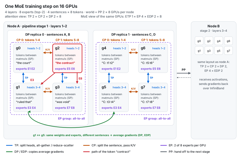
The whole layout in one picture. Rows inside a replica are TP ranks (heads), columns are CP ranks (halves of the sentence), the two replicas are DP copies, and each dashed purple box is one EP group holding all 8 experts. Red is the token “contract”; green links GPUs that average gradients; node B repeats the layout for layers 3–4.
The setup: one MoE model, one batch, 16 GPUs
Model: 4 layers. Each layer = attention with 4 heads, then an MoE layer with 8 experts (E1–E8), each token picks its top 2. Plus the embedding at the start and the output head at the end.
Batch: 4 sequences of 8 tokens each (32 tokens). Sequence A is “the court ruled that the contract was void”: t1 = the, t2 = court, … t6 = contract, t7 = was, t8 = void. Sequences B, C, D are other sentences.
Hardware: 2 nodes × 8 GPUs = 16 GPUs. Inside a node, GPUs talk over NVLink (fast); between nodes over InfiniBand (slower).
The layout, chosen so every parallelism shows up:
world = 16 GPUs = PP 2 × 8 GPUs per stage
attention view of a stage:  TP 2 × CP 2 × DP 2   = 8
MoE view of the same stage: ETP 1 × EP 4 × EDP 2 = 8
The rule that always holds: both views must multiply to the same number of GPUs, because they are two ways of labelling the same 8 GPUs.
Which GPU holds what? The map
Node A runs pipeline stage 1 (layers 1–2); node B runs stage 2 (layers 3–4) with exactly the same layout. Inside node A:
                 DP replica 0 (seqs A, B)        DP replica 1 (seqs C, D)
                 CP rank 0      CP rank 1        CP rank 0      CP rank 1
                 tokens 1–4     tokens 5–8       tokens 1–4     tokens 5–8
TP rank 0        g0             g2               g4             g6          heads 1–2
TP rank 1        g1             g3               g5             g7          heads 3–4

MoE view of the same GPUs (ETP 1, EP 4, EDP 2):
                 EP group 0                       EP group 1 (an EDP copy of group 0)
experts held     g0: E1 E2   g1: E3 E4            g4: E1 E2   g5: E3 E4
                 g2: E5 E6   g3: E7 E8            g6: E5 E6   g7: E7 E8
Read it like this. DP picks the sequences (column pair). CP picks which half of the sequence (column). TP picks which heads (row). For the MoE layer, the same GPUs are relabelled: within each group of 4, GPU k holds 2 of the 8 experts, and the second group of 4 holds a full copy.
Every group in node A (communication only happens inside these):
TP groups    {g0,g1} {g2,g3} {g4,g5} {g6,g7}     same tokens, different heads
CP groups    {g0,g2} {g1,g3} {g4,g6} {g5,g7}     same heads, different halves of the sequence
DP groups    {g0,g4} {g1,g5} {g2,g6} {g3,g7}     same weights, different sequences
EP groups    {g0,g1,g2,g3} {g4,g5,g6,g7}         different experts, swap tokens
EDP groups   {g0,g4} {g1,g5} {g2,g6} {g3,g7}     same experts, different tokens
PP pairs     g0(node A)–g0(node B), g1–g1, …     layers 1–2 hand off to layers 3–4
Step 1: DP and PP: who gets which data, and in what order
DP splits the batch: replica 0 (g0–g3) gets sequences A and B, replica 1 (g4–g7) gets C and D. Both replicas hold the same weights.
PP splits the layers: node A runs layers 1–2, node B runs layers 3–4. To keep both nodes busy, each replica feeds its 2 sequences as 2 micro-batches: micro-batch 1 = sequence A (and C on replica 1), micro-batch 2 = B (and D).
time →        slot 1         slot 2         slot 3
node A        A fwd L1–2     B fwd L1–2     (backward work)
node B        idle           A fwd L3–4     B fwd L3–4
                             ↑ node A sends A's activations to node B (point-to-point)
The idle slot is the pipeline bubble. More micro-batches make it a smaller share of the step.
Step 2: CP and TP + SP: where do sequence A’s tokens sit?
CP splits the sequence for the whole layer: on replica 0, CP rank 0 gets t1–t4 (“the court ruled that”), CP rank 1 gets t5–t8 (“the contract was void”).
TP splits the attention weights: in each TP pair, one GPU computes heads 1–2 and the other heads 3–4, for the same tokens.
SP splits tokens again, but only between TP’s matrix multiplies (LayerNorm, residual adds, and the MoE layer). So where a token lives depends on the moment:
                     inside attention (TP)      between matmuls (SP), incl. MoE
g0  TP0, CP0         A: t1–t4, heads 1–2        A: t1 t2   "the court"
g1  TP1, CP0         A: t1–t4, heads 3–4        A: t3 t4   "ruled that"
g2  TP0, CP1         A: t5–t8, heads 1–2        A: t5 t6   "the contract"
g3  TP1, CP1         A: t5–t8, heads 3–4        A: t7 t8   "was void"
g4–g7                same for sequence C
So “contract” (t6) lives on g2. Every GPU in a DP replica holds a different slice of the same sequence, and no work is duplicated.
Step 3: follow “contract” through attention in layer 1
g2 holds the hidden states of “the” and “contract” (its SP slice) and applies LayerNorm locally.
SP all-gather in the TP pair {g2, g3}: now both hold t5–t8, the full CP half, because each computes some heads for all of them.
g2 computes Q, K, V for heads 1–2; g3 for heads 3–4. No communication: each GPU has its own columns of the weight matrices (column-parallel).
CP ring: “contract” must attend to t1–t4 too, whose K and V sit on g0 (same heads, other half). g0 passes its K, V for heads 1–2 to g2; g1 does the same for g3. Causal masking: t1–t4 never look at t5–t8, so g0 has less work than g2. Real systems fix this by giving each CP rank one early and one late chunk (rank 0: t1 t2 t7 t8, rank 1: t3–t6).
Output projection (row-parallel): g2 and g3 each produce a partial sum over their heads. SP reduce-scatter adds them and hands back the token slices: g2 gets the finished t5 t6, g3 gets t7 t8.
g2 "the contract" → all-gather(TP) → heads 1–2 for t5–t8 ⇄ K,V ring with g0 (CP)
                 → reduce-scatter(TP) → g2 "the contract", attention done
Step 4: follow “contract” through the MoE layer: EP, ETP, EDP
Route: g2 runs the router (a small matrix every GPU has) on its two tokens. “the” → E1, E2. “contract” → E3 (gate 0.6), E8 (gate 0.4).
Dispatch (EP all-to-all in {g0, g1, g2, g3}): E1, E2 live on g0, E3 on g1, E8 on g3. g2 sends “the” to g0 once (both its experts are there), and “contract” to g1 and g3. Every GPU in the group does the same with its own tokens at the same moment.
Compute: g1 now holds every token from sequence A that chose E3 or E4, and runs E3 and E4 on them as one batched matrix multiply. ETP = 1 means each expert is whole on one GPU; no expert is split.
Combine (all-to-all back): the E3 output returns from g1 and the E8 output from g3 to g2, which computes contract_out = contract + 0.6·E3(contract) + 0.4·E8(contract).
g2 ─"contract"→ g1 (E3) ─┐
   ─"contract"→ g3 (E8) ─┴→ back to g2: 0.6·E3 + 0.4·E8 + residual
   ─"the"─────→ g0 (E1, E2) → back to g2
Meanwhile g4–g7 do exactly the same for sequence C with their own copy of E1–E8. That second copy is EDP: same experts, different tokens. The two copies only talk at the end of the step, to average gradients.
Why SP matters here: after the reduce-scatter, each GPU holds different tokens, so each routes only its own. Without SP, g2 and g3 would both hold t5–t8 and both would send “contract” to E3: double the traffic and work.
Then layer 2 repeats steps 3 and 4. After layer 2, g2 sends its slice (“the contract”) to g2 on node B: the PP handoff, the only traffic between nodes.
Step 5: backward pass and gradient sync: who averages with whom?
Backward runs the same path in reverse: node B sends gradients back to node A (PP), all-gather and reduce-scatter swap places (TP/SP), the CP ring passes K/V gradients back, and the two all-to-alls run in reverse (EP).
Then every weight’s gradient must be averaged over all GPUs that hold a copy of that weight and saw different tokens:
weight (stage 1)          copies on                  gradient all-reduce over
attention heads 1–2       g0, g2, g4, g6             DP × CP   {g0,g2,g4,g6}
attention heads 3–4       g1, g3, g5, g7             DP × CP   {g1,g3,g5,g7}
experts E1, E2            g0, g4                     EDP       {g0,g4}
experts E3, E4            g1, g5                     EDP       {g1,g5}
LayerNorm, router         all 8                      all 8     (TP × CP × DP)
Why CP is in the attention group: g0 and g2 hold the same heads but saw different tokens (t1–t4 vs t5–t8), so their gradients are partial and must be added. Same idea for SP-split LayerNorm and router weights across the TP pair.
Note the two groups: attention gradients average over 4 GPUs, expert gradients over 2. Getting either group wrong gives silently wrong training, not a crash.
Finally the optimizer step. With ZeRO-1, the Adam states for heads 1–2 are split 4 ways across g0, g2, g4, g6, and for E1, E2 split 2 ways across g0, g4.
The one-table summary of every parallelism in the example
name    splits                    in the example                    group   communication
DP      the batch                 seqs A,B on g0–3; C,D on g4–7      2       gradient all-reduce, once per step
ZeRO-1  optimizer state           Adam states split over copies      —       reduce-scatter + all-gather, once per step
PP      layers                    layers 1–2 node A, 3–4 node B      2       point-to-point activations, at the cut
TP      attention weights         heads 1–2 vs 3–4                   2       all-gather + reduce-scatter, every layer
SP      tokens between matmuls    "the contract" vs "was void"       = TP    (same collectives as TP)
CP      tokens through attention  t1–t4 vs t5–t8                     2       K/V ring, every attention layer
EP      experts                   2 of 8 experts per GPU             4       all-to-all ×2, every MoE layer
ETP     each expert's matrices    not split                          1       none
EDP     copies of the experts     g0–3 vs g4–7                       2       expert gradient all-reduce, once per step
What g2 stores: half of the attention weights of layers 1–2 (TP 2, PP 2 → one quarter of all attention), experts E5, E6 of layers 1–2 (one eighth of all experts), a full copy of LayerNorms and routers for layers 1–2, a share of the optimizer states, and activations for 2 tokens of sequence A between matmuls (4 inside attention).
Traffic by link: TP, SP, CP and EP all stay inside a node on NVLink; only PP crosses InfiniBand, carrying a small slice of activations. That is the usual design: the chattiest parallelisms go innermost.
What changes with other settings, and an everyday analogy
No SP: g2 and g3 both hold t5–t8 at the MoE layer and both route them, so every token is sent and computed twice. Megatron refuses to train MoE with TP > 1 without SP.
ETP 2 (EP 2, EDP 2): each expert’s matrices are split across a pair of GPUs, and the pair must add partial results after every expert. Fine-grained experts are already small, so this mostly adds communication. Usually ETP = 1.
EP 8 (EDP 1): one expert per GPU and no expert copies. Less expert memory per GPU, but the all-to-all now spans both DP replicas (all 8 GPUs), and one hot expert slows all 8.
PP 1 with DP 4: every GPU holds all 4 layers (twice the weights) but there is no bubble and no inter-node activations; the gradient all-reduces now cross nodes instead.
Analogy, a restaurant: orders are sequences. DP = two identical kitchens, each taking half the orders. PP = an assembly line, prep station (node A) then finishing station (node B), with orders passed along. TP = two cooks splitting one dish’s steps. SP = between steps, the cooks split the plates instead. CP = a huge order split between cooks who swap notes. EP = specialist chefs (grill, pastry): each plate goes to its two specialists and comes back. EDP = each kitchen has its own set of specialists, who compare notes at closing. ETP = two chefs sharing one specialty, rarely worth it.
Cheat sheet
| Method | Splits | Communication | Main limit |
|---|---|---|---|
| DP | batch | all-reduce of gradients | full model per GPU |
| ZeRO-1/2/3 | optimizer state / + grads / + weights | reduce-scatter, all-gather | ZeRO-3 moves weights every step |
| TP | weight matrices | 4 all-reduces per layer | must stay inside a node; heads ÷ t |
| SP | tokens between TP matmuls | reduce-scatter + all-gather (same bytes as TP) | size = TP size |
| CP | tokens through the whole layer | K/V around a ring | causal imbalance, custom masks |
| PP | layers | point-to-point activations | bubble = (p − 1)/(m + p − 1) |
| EP | MoE experts | all-to-all of tokens, twice per MoE layer | slowest GPU sets the pace; needs load balancing |
References
- Shoeybi et al., Megatron-LM, 2019. arXiv:1909.08053
- Korthikanti et al., Reducing Activation Recomputation in Large Transformer Models, 2022. arXiv:2205.05198
- Liu et al., Ring Attention with Blockwise Transformers, 2023. arXiv:2310.01889
- Dao et al., FlashAttention, 2022. arXiv:2205.14135
- Huang et al., GPipe, 2018. arXiv:1811.06965
- Narayanan et al., Efficient Large-Scale Language Model Training on GPU Clusters Using Megatron-LM, 2021. arXiv:2104.04473
- Qi et al., Zero Bubble Pipeline Parallelism, 2023. arXiv:2401.10241
- Rajbhandari et al., ZeRO, 2019. arXiv:1910.02054
- DeepSeek-AI, DeepSeek-V3 Technical Report, 2024. arXiv:2412.19437
- Lepikhin et al., GShard, 2020. arXiv:2006.16668
- Fedus et al., Switch Transformers, 2021. arXiv:2101.03961
- Rajbhandari et al., DeepSpeed-MoE, 2022. arXiv:2201.05596
- Gale et al., MegaBlocks, 2022. arXiv:2211.15841
- Liu et al., MoE Parallel Folding, 2025. arXiv:2504.14960